I encountered this problem while exploring a compact cycling power meter, where the sensor had to fit into the tiny cavity of a bike spindle and the available mechanical deformation was so small that conventional measurement approaches became challenging. This led me to investigate an optical approach to torque measurement.

Purpose of the Project

The ultimate goal of this project was the realization of a torque sensor that could fit into the tiny hollow cavity of a shaft.

Such a sensor could enable applications ranging from torque feedback for closed-loop control of robotic joints and actuators to load monitoring and condition-based maintenance of mechanical systems.

The insertion of the sensor into a tiny cavity presents an important advantage: it can retrofit onto existing hardware without being invasive.

Technical Aspects: Torque Measurement

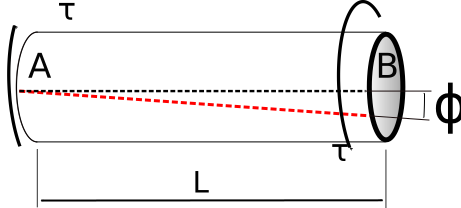
An accurate estimation of the torque $\tau$ traversing a shaft is quite challenging. For high accuracy measurements, a sensor needs to detect microscopic deformations (angle of twist) of the shaft undergoing mechanical stress.

As shown in Fig. 1, a torque applied to a shaft induces two separate cross-sections A and B to twist respectively by an angle $\phi$.

Their relationship is described by the following equation:

$$ \phi = \tau \, \frac{L}{G \cdot J} $$

where:

• $\phi$ is the angle of twist between the two distinct sections A and B;
• $\tau$ is the applied torque;
• $L$ is the distance between the sections A and B;
• $G$ is the shear modulus or modulus of rigidity of the material, which is a property of the material;
• $J$ is the polar moment of inertia of the shaft, defined as $J \overset{\mathrm{def}}{=} \iint \limits_A \rho^2 \, dA$, where $\rho$ is the distance to the element $dA$;

For a regular geometry, such as a cylindrical hollow shaft, the polar moment of inertia along its rotational axis is:

$$ J = \frac{\pi}{2} (r_2^4 - r_1^4) $$

where $r_2$ and $r_1$ are the external and the internal radius, as Fig. 2 depicts.

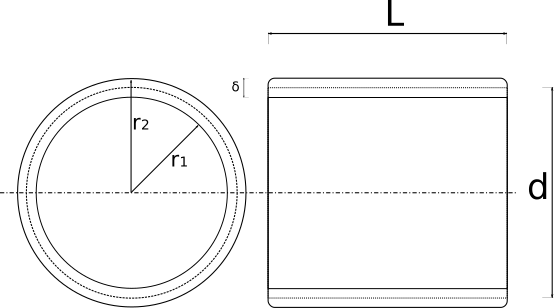
By considering instead the mean diameter $d$ and the thickness $\delta$ as parameters, the above equation rewrites into:

$$ J = \frac{\pi}{2} \left(\left(\frac{d + \delta}{2}\right)^4 - \left(\frac{d - \delta}{2}\right)^4\right) = \frac{\pi}{4} \, d \, \delta \, (d^2 + \delta^2) $$

In case of a relatively thin radial surface $\delta$ compared to the mean diameter $d$ — i.e., $\delta = k \cdot d$, with $0 < k \ll 1$ — the above equation simplifies to:

$$ J = \frac{\pi}{4} \, d^3 \, \delta $$

with a relative error $\frac{k^3}{k + k^3} \approx k^2$.

To reach a resolution suitable for control-loop applications, the sensor should be able to detect torque changes on the order of $1\,Nm$.

For example, considering a stainless-steel shaft (shear modulus $G = 77.2 \cdot 10^9\,Pa$) with external diameter $30\,mm$, thickness $3\,mm$ and shaft segment length $L = 50\,mm$, the resulting angle of twist is approximately $7.90 \cdot 10^{-4}$ degrees, i.e., on the order of $10^{-3}$ degrees.

Working Principle

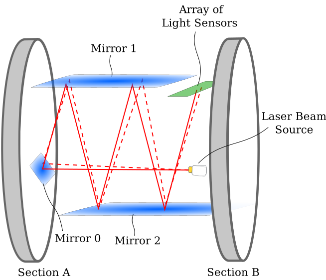
Figure 3 illustrates the torque sensor's working principle. The two distinct cross-sections A and B twist with respect to each other whenever a torque is applied to the shaft. A laser beam is generated and reflected by Mirror 0 towards Mirror 1. The latter is rigidly connected to section A. Similarly, the third mirror (Mirror 2) is rigidly connected to section B. The laser beam is repeatedly reflected between the two mirrors 1 and 2. When sections A and B rotate relative to each other by an angle $\phi$ (see Fig. 4 to the right), a corresponding misalignment between mirrors 1 and 2 occurs. Such a misalignment causes a deviation of the laser beam, as shown on the right of Fig. 4. By measuring the deviation $S(\phi)$ of the laser beam by means of an array of light sensors, it is possible to infer the relative rotation of sections A and B (i.e., the angle $\phi$). As the distance L between sections A and B is known, as well as the parameters G and J, the torque $\tau$ results from the angular twist equation. The measurement can be amplified by adjusting the deflection of mirror 0, in order to control the number of reflections of the laser beam between mirrors 1 and 2.

The key idea is therefore not to measure the microscopic angular deformation directly. Instead, the mechanical deformation is converted into an optical displacement that can be measured more easily. By changing the optical geometry and, in particular, the number of reflections, the measurement gain can be adjusted without changing the sensing element itself.

A microscopic mechanical deformation can be converted into a measurable optical displacement, while the optical geometry itself provides a way to control the measurement gain.

Computer Simulation

A preliminary check of the above approach, before building a prototype, was carried out through computer simulation. A custom simulator creates the beam reflection and estimates the expected deflection seen by a linear array sensor. Results indicate that for a tiny variation of the angle $\phi$, it is possible to amplify the signal to detect variation of $S(\phi)$ with a low-resolution linear array sensor (TSL1401CCS, 128x1 pixels, 400 DPI, ams.com/tsl1401ccs).

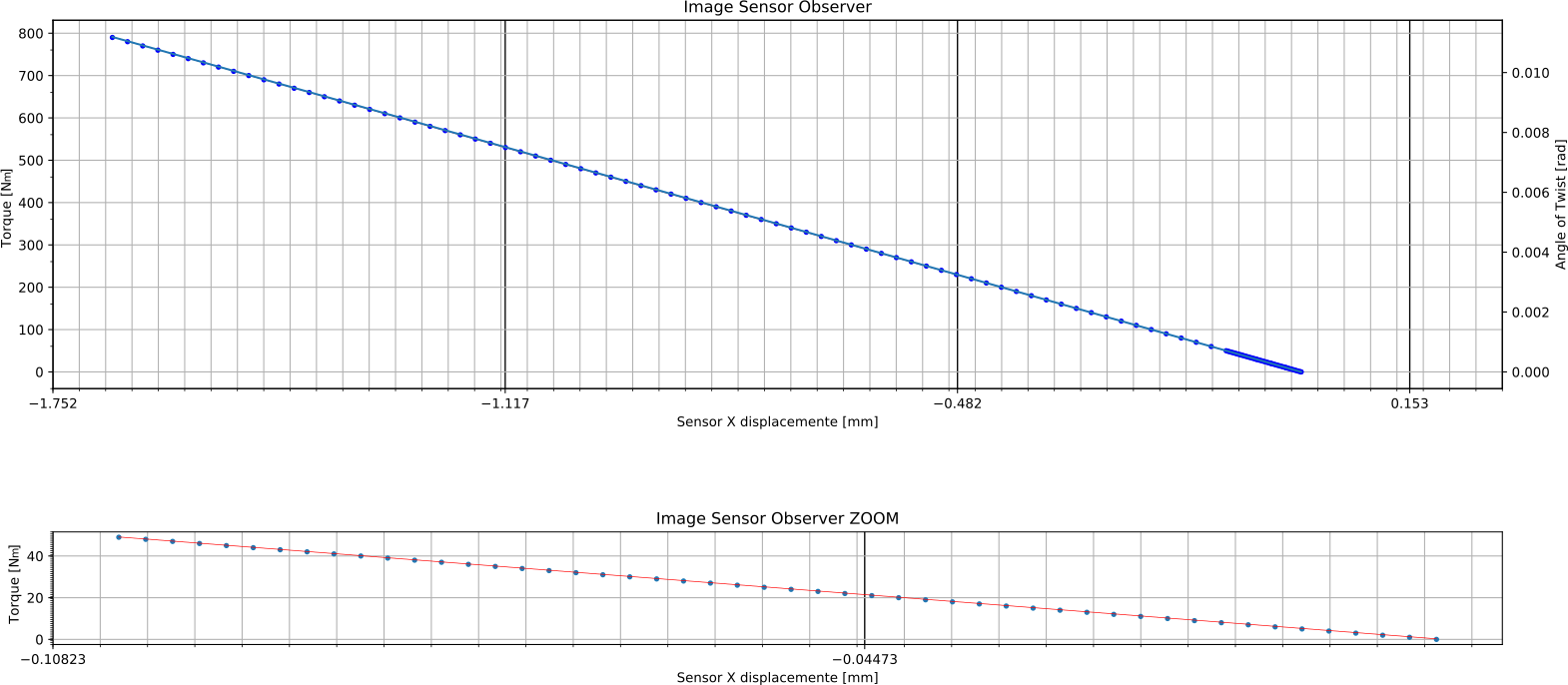
The graph reported in Fig. 5 shows the relationship between the applied torque and the displacement of the laser beam detected by the sensor. Each interval along the X-axis corresponds to 5 pixels of the linear array sensor. By interpolating the light intensity measured by the linear array sensor, we expect to be able to estimate torque with an accuracy of 1 Nm. The graph below corresponds to a stain-steel shaft with external diameter 24.4 mm, thickness 7 mm and segment lenght 32 mm. The computer simulation relies on the beam reflection model described in the next section.

Beam Reflection Model

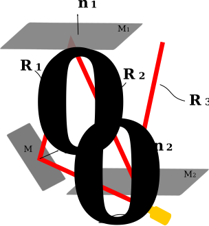
The general equation describing the reflection $\vec{r}$ of a laser beam $\vec{b}$ against a mirror perpendicular to the vector $\vec{m}$ is:

$$ \vec{r} = \vec{b} - 2 \frac{\vec{b} \cdot \vec{m}}{\| \vec{m} \|^2} \cdot \vec{m} $$

The above equation, valid for the 3D case, can be generalized to model consecutive reflections $\vec{R_i}$ of a laser beam against a sequence of mirrors $\{M_0, M_1, \dots, M_j\}$, as Fig. 6 above instantiates. The $i$-th reflection $\vec{R_i}$ reflects against the mirror $M_j$, generating the ray $\vec{R_{i+1}}$. For each mirror $M_j$, we consider the versor $\vec{n_j}$ perpendicular to the reflecting surface of the mirror $M_j$. This way, the general reflection equation results in the following recurrence:

$$ \vec{R_{i+1}} = \vec{R_i} - 2 \left( \vec{R_i} \cdot \vec{n_j} \right) \cdot \vec{n_j} $$

with $\vec{R_0}$ being the source beam output by the laser.

A more convenient representation of this recurrence allows us to solve it. A preliminary observation is that the dot product of three vectors $(\vec{a} \cdot \vec{b}) \cdot \vec{c}$ can be rearranged as $(\vec{c} \cdot \vec{b}^\top) \cdot \vec{a}$. By applying this property to the three-vector dot product above and rearranging the terms, we obtain:

$$ \vec{R_{i+1}} = (I - 2 \cdot \vec{n_j} \cdot \vec{n_j}^\top) \cdot \vec{R_i} = (I - 2 \cdot N_j) \cdot \vec{R_i} $$

where $I$ is the identity matrix and $N_j$ the outer (or tensor) product $N_j \stackrel{\text{def}}{=} \vec{n_j} \otimes \vec{n_j} = \vec{n_j} \cdot \vec{n_j}^\top$.

An assumption we can make for the practical application of this equation is that the sequence of mirrors hit by the beam is known in advance. Although for programming a simulation this assumption is too restrictive, for the following discussion it is sufficient. The inclination of $M_0$ determines the number of reflections of the beam against $M_1$ and $M_2$, hence the sequence of mirrors. For example, looking back to the working-principle (Fig. 3), the sequence $\{M_0, M_1, M_2, M_1, M_2\}$ is known.

$$ \vec{R_{i+1}} = \begin{cases} (I - 2 \cdot N_0) \cdot \vec{R_0} & \text{if } i = 0, \\ (I - 2 \cdot N_1) \cdot \vec{R_i} & \text{if } i > 0 \text{ is odd} \\ (I - 2 \cdot N_2) \cdot \vec{R_i} & \text{if } i > 0 \text{ is even} \end{cases} $$

which, for the depicted case, results in:

$$ \vec{R_{i+1}} = (I - 2 \cdot N_2) \cdot (I - 2 \cdot N_1) \cdot (I - 2 \cdot N_2) \cdot (I - 2 \cdot N_1) \cdot (I - 2 \cdot N_0) \cdot \vec{R_0} $$

Beam Reflection Point

To compute the exact point at which the beam reflects or hits a surface (i.e., mirror or sensor), we consider the intersection between the beam and the mirror. The problem can be algebraically solved by considering the intersection between a line and a plane. For each mirror $M_j$, the normal versor $\vec{n_j}$ is known. In vector notation, the equation of a mirror (plane) is the set of points $\vec{p}$ such that $(\vec{p} - \vec{M_j}) \cdot \vec{n_j} = 0$, where $\vec{M_j}$ is a known point of the mirror. Similarly, the equation of the $i$-th beam (line) is the set of points $\vec{p}$ such that $\vec{p} = l \vec{R_i} + \vec{R_i^0}$, where $\vec{R_i^0}$ is a known point of the beam. By combining the two equations, $(l \vec{R_i} + \vec{R_i^0} - \vec{M_j}) \cdot \vec{n_j} = 0$, we first solve for $l$ and calculate the intersection as:

$$ \vec{p} = \frac{(\vec{R_i^0} - \vec{M_j}) \cdot \vec{n_j}}{\vec{R_i} \cdot \vec{n_j}} \, \vec{R_i} + \vec{R_i^0} $$

The simulation process also requires checking whether the point $\vec{p}$ belongs to the mirror $M_j$.

Considerations

The optical measurement itself is inherently insensitive to electromagnetic interference, including RF sources such as Wi-Fi. Temperature, however, remains a mechanical error source: expansion or contraction of the material supporting the mirrors, and of the mirrors themselves, might introduce noise in the measurement. However, compared to the majority of existing solutions, which are typically based on strain gauges — hence very temperature-dependent — the influence that temperature has on this device is potentially negligible.

From Simulation to Real Prototype

Moving from simulation to a real prototype surfaces three engineering trade-offs.

1. Accuracy vs. low-cost optical components

The costs of the optical components required to obtain the desired accuracy play a relevant role. Collimated high-end laser sources, for example, would guarantee accurate results; similarly, custom first-surface optical mirrors would provide smooth and sharp reflections. However, their costs — also for large quantities — can be prohibitive. The open question this prototype needs to answer is whether it is possible to detect displacements with high accuracy (10 nm) using low-cost optical components.
Eventually, the mirrors themselves were cut from a reflective plastic board salvaged from a toy — good enough reflectivity for a first proof-of-concept, well before sourcing proper first-surface mirrors.

2. Universal compatibility via expandable rings

The internal diameter and shape of the target shafts can vary quite significantly. To provide a universal, easy-to-install solution, the sensor body is equipped with expandable rings, which adapt to different shafts regardless of their diameters and internal shapes.

However, it is particularly challenging to design an expandable ring that engages the narrow cavity of the shaft and locks the sensor in place. Even microscopic deformations of the shaft at the interface with the expandable ring might compromise both the accuracy and the precision of the measurement. To prevent this undesired effect, or at least to minimize its impact, optimal design and accurate material selection, supported by repeated lab tests, are necessary to progressively refine the design and achieve a reliable solution.

3. Batteryless, practical, and eco-friendly power

One temptation is to design the sensor around an onboard battery, for applications where the target shaft rotates continuously. This has three major drawbacks: first, it requires the user to periodically recharge or change the battery; second, batteries contain disposable substances harmful to the environment; third, the narrow cavity of the shaft constrains the dimensions of the battery, hence its capacity. An alternative is to harvest clean energy by exploiting the rotation of the shaft itself, and to temporarily store it in a super capacitor for a batteryless device. The main challenge is to provide a continuous and sufficient source of energy, even in spite of irregular rotation, as if it were battery powered.

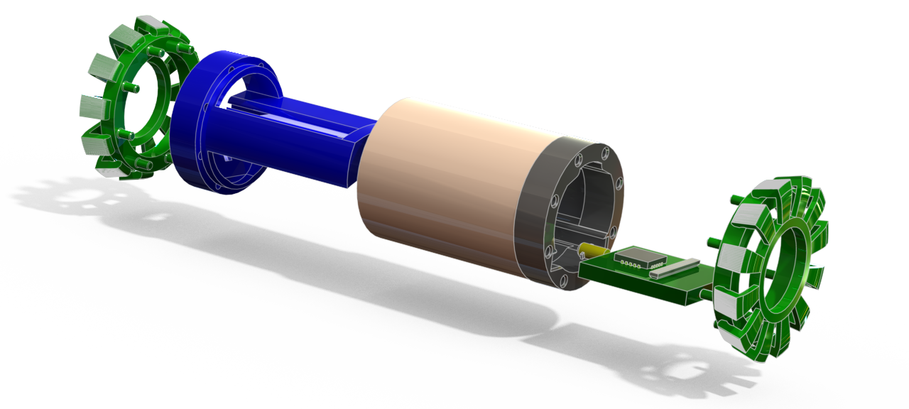
The prototype depicted in the picture above includes the minimal components for testing the idea:

• the sensor enclosure, to hold the mirrors and the electronics;
• the electronic board, embedding a light sensor array to detect beam deflection, the laser beam source, and the MCU;
• the expandable rings, for installation into a real shaft.

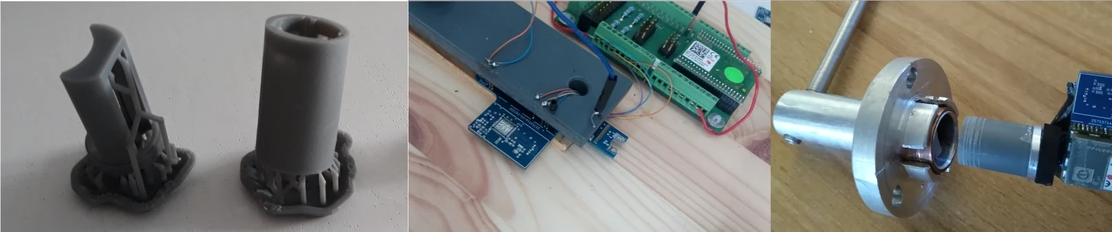
Figure 8 shows the 3d printed parts composing the body. They are printed on a resin machine. The first prototype was laid out on an extended board that could fit into the target shaft while still allowing external interface and probe connections with ease. This prototype does not include a capacitor for storing energy, since the focus at this stage is on assessing accuracy and feasibility. The central picture of Fig. 8 shows the board protruding from a plastic holder that is mainly used to program and test the initial firmware. The tiny light array is visible on the board, while the laser source is not yet mounted. The picture on the right shows the fully assembled sensor, inserted in an 18 mm diameter pipe with a ring fixture and a lever to apply a torque manually for testing the complete assembly. An attempt to build the expandable rings displayed in Fig. 7 was made with an FDM 3D printer. Probably due to the choice of material or printer settings, the results weren't satisfactory.
For testing the sensor, a rigid metal ring perfectly tailored to the target shaft was machined from a thick aluminium pipe.

Prototype Validation

The first prototype was built to validate the measurement architecture and identify the main practical limitations of the design.

The prototype integrated the optical system, linear light sensor, microcontroller, electronics and mechanical enclosure into a compact assembly. It was installed inside a test shaft and manually loaded to induce a small torsional deformation.

The experiment confirmed the expected behavior: the laser beam reached the light-sensor array through the intended sequence of reflections, and the sensor output varied when torque was applied to the shaft. The observed behavior was consistent with the response predicted by the simulation.

A quantitative characterization of accuracy is not available. The prototype should therefore be considered a feasibility prototype rather than a fully characterized torque sensor.

Final Consideration

The simulation and subsequent prototype demonstrate the feasibility of the sensing concept.

The innovation wasn't simply replacing a strain gauge with an optical sensor. It was using the optical path itself as a controllable gain mechanism.

The work started from a cycling power-meter application, but the underlying sensing architecture is applicable to a broader class of compact mechanical systems where torque must be measured without significantly modifying the load-bearing structure.

Recognizing the novelty of the project, Science Park Graz (SPG), an Austrian high-tech incubator, supported its development, while the Austrian Research Promotion Agency (FFG) provided a grant covering the patent-related expenses.

Eventually, the Austrian Patent Office granted the patent AT525176B1 in 2023.