From Mathematical Abstraction to Heterogeneous Robotic Platforms

During my PhD, I modelled long chains of modular robots¹ as collections of coordinate frames connected through homogeneous transformations. At the time, I considered it simply a robotics problem. Years later, while designing industrial validation systems, I realized the same mathematical abstraction could solve a completely different challenge. Instead of describing only the robot, the transformation graph could describe the entire automation environment. That small change in perspective becomes the foundation of a software architecture that remains stable while the hardware evolves.

Key Takeaway

Mathematical abstraction lays the foundation for software longevity

Robotic systems become reusable when software describes objectives and configurations rather than machine-specific operations. By using coordinate transformations and kinematic abstraction, the same software framework can control completely different robotic architectures — from single-axis actuators to Cartesian systems and six-degree-of-freedom robots.

---

Preamble

This article is a deliberate generalization of a real-world case study from one of my engineering engagements. To preserve confidentiality, I've replaced the specific application with a representative stand-in — the underlying engineering challenge and architectural principles are unchanged.

To guide the following explanation, we consider the following task: test the sensitivity, responsiveness, and accuracy of a touchscreen as a pencil approaches and touches it along different trajectories.

---

Introduction: Validation of Complex Electronic Systems Is a Physical Challenge

Validation of complex electronic systems is not limited to firmware execution, communication protocols, or electrical measurements. Many real-world conditions require physical interaction — a pencil drawing on a touchscreen, for instance, requires actual physical actuation, not just a signal on a wire.

In practice, these validation platforms are often assembled from repurposed motion hardware — a spare CNC gantry or 3D printer chassis pushed well beyond its original intent — because the mechanical structure is a solved problem. It's cheap, available, and well understood. The software architecture around it usually isn't.

That gap is the real subject of this article. A modern validation platform is a combination of robotic architectures, measurement equipment, tools, and a test framework controlling the whole system. The main challenge is that over time the devices under test, the testing tools — like probes, such as the pencil in our touchscreen example — and the platform itself keep evolving. The system architecture has to accommodate upcoming use cases while remaining backward compatible with the ones it already supports.

A poorly designed automation system usually responds to this evolution by accumulating exceptions: hardcoded robot coordinates, scripts tied to one hardware variant, dedicated logic bolted on for each new machine. Every hardware change becomes a software modification, and the codebase slowly turns into a record of every machine it has ever had to support, rather than a description of what the tests are actually trying to do.

A robust automation platform requires the opposite approach: separate what the machine is from what the system should do. A test should describe engineering intent — "place this pencil at this location relative to the device" — rather than machine commands: "move this motor by 1250 steps."

The Hardware Diversity Problem

Different validation requirements naturally lead to different robotic architectures. The following table illustrates a few examples:

Test requirement	Required capability	Simplest robot
Move probe along one axis	Linear positioning	1 DOF
Reach multiple positions on one plane	Planar positioning	3 DOF Cartesian
Handle multiple probes	Tool exchange / multi-probe fixture	3 DOF Cartesian
Reach arbitrary orientations	Full spatial positioning	6 DOF

This raises an obvious question: should every validation station simply use the most capable robot available? A six-axis arm could, in principle, solve every problem on this list. But engineering decisions involve more than raw capability — cost, maintenance, footprint, complexity, and throughput all push in the other direction. In many industrial environments, a simpler machine is the better engineering choice whenever it's sufficient for the job.

Which leaves the real challenge: how can the same software framework control completely different robotic architectures, without rewriting it for each one?

From Software Modularity to Geometric Abstraction

Robust software engineering builds on modularity and abstraction. Each physical and virtual component can be represented by a dedicated software module: robots expose motion capabilities, tools — a probe, such as our touchscreen pencil, is one example — expose physical and electrical interfaces, fixtures define mechanical constraints, and test sequences coordinate operations between them. Tools, devices, and fixture variants can be defined through class inheritance and composition; test sequences become macro operations controlling each component at a specific point in time; synchronization between subsystems can rely on events, shared state, and message passing.

Object-oriented abstraction can also represent the hierarchical interconnection among physical components — but this is where the difficulty actually starts, because representing components isn't the same as computing where they are in space. The obvious approach is to recursively compute the position and orientation of each component relative to the one it's attached to, walking the object hierarchy at runtime. In my experience, this runs into trouble quickly: it degrades performance and scalability, and the software complexity grows faster than the system it's meant to describe.

A better approach takes one step back and looks at the system as a whole rather than component by component. The kinematics of the system result from the combined geometries of the interconnected components, and that reframing changes what "changing a component" actually means:

• Modifying a fixture changes the device position, which introduces an offset in the tool actuation chain;
• Swapping a probe changes the tip location, which requires the robot's end-effector motion to compensate accordingly;
• Changing the robot architecture affects the reachable workspace and the kinematics, which affects every motion routine downstream.

Each of these is a local change with a system-wide consequence — which is exactly the kind of relationship chained coordinate transformations are built to handle. A solid and elegant solution abstracts the geometric relationships this way and lets algebraic computation, rather than object traversal, do the work of resolving the kinematics.

Frames of Reference Transformations

Bodies can be mathematically described as a set of frames of reference, corresponding to their physical connectors to other bodies. Frames of reference are geometrically linked via coordinate transformations, so that interconnected bodies can be spatially described through a chain — more generally, a tree — of relative transformations: a fixture relative to the workspace, a device relative to the fixture, a probe relative to the end-effector, the end-effector relative to the robot base.

The complete system can be depicted as a graph of coordinate transformations, as in the picture below:

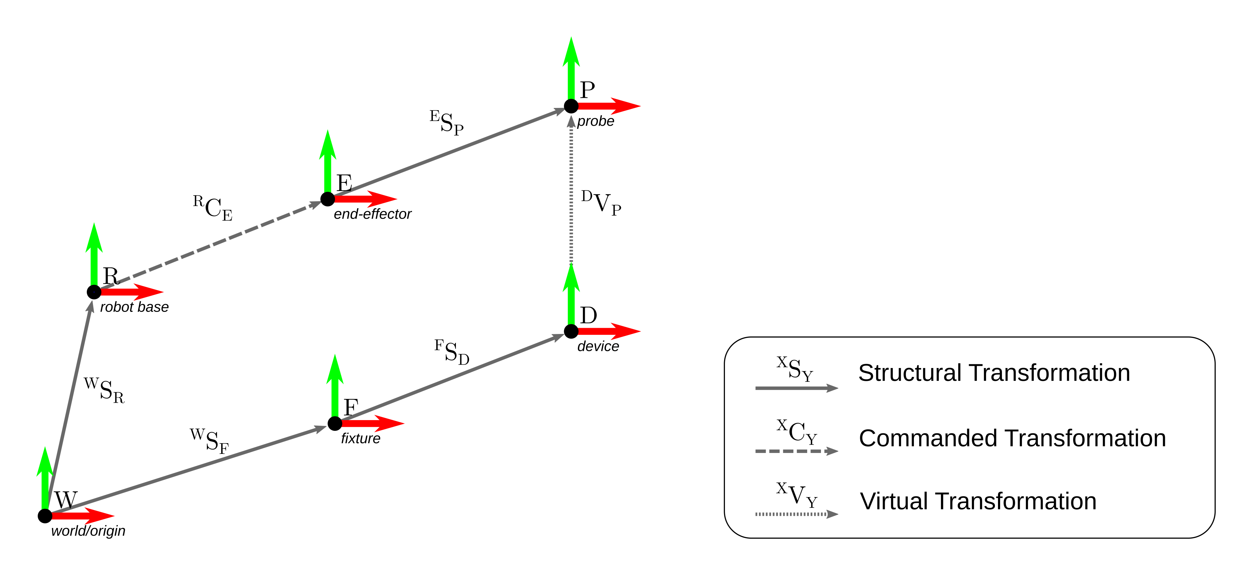
The notation $^XS_Y$ represents the coordinate transformation of frame Y expressed with respect to frame X. These transformations fall into three categories, each describing a different kind of relationship:

Structural transformations ($^XS_Y$) describe physical, rigid characteristics — fixture dimensions, probe geometry, mechanical mounting relationships. They don't change unless the hardware itself does.

Control transformations ($^XC_Y$) describe the robot end-effector position with respect to the robot base. They abstract away the robot's specific kinematics entirely, providing a universal reference regardless of whether the robot underneath is a single actuator or a six-axis arm.

Virtual transformations ($^XV_Y$) provide convenient reference frames that don't correspond to physical hardware at all — device checkpoints, test locations, calibration references.

The Loop Equation

The strength of this approach comes from a simple fact: every closed transformation loop creates a mathematical constraint. Because two different paths through the graph must arrive at the same physical point, they can be set equal to each other — and that equality is what lets the system solve for an unknown.

For example:

$$ ^WS_R \cdot ^RC_E \cdot ^ES_P = ^WS_F \cdot ^FS_D \cdot ^DV_P$$

On the right-hand side, everything is known: the structural transformations describe fixed geometry, and $^DV_P$ describes the desired final positioning of the probe relative to the device — the outcome we actually want. On the left-hand side, the structural transformations are again known, but $^RC_E$ — the robot base-to-end-effector transformation — is not. Solving the equation for it is what tells the robot where to go, since this single transformation contains everything needed to control it.

Specifically, the coordinates of the end-effector origin relative to the robot base give the robot pose in Cartesian coordinates:

$$ ^RC_E \cdot \begin{bmatrix} 0 \\ 0 \\ 0 \\ 1 \end{bmatrix} = f(q) $$

where $f(q)$ is the robot control in joint coordinates, and the inverse kinematics needed to compute $q = f^{-1}$ belongs to the robot's own API — not to this framework.

That division of labor is the point: the robot controller becomes an implementation detail, hidden behind a single high-level command:

probe.move_to(device_rel_pose)

This one call can drive a linear stage, a Cartesian gantry, or a six-axis arm without any change to the calling code. The software above it never touches motors or joints directly — it solves geometric relationships, and lets each robot's own controller translate the result into motion.

From Static Pose to Trajectory

The loop equation as written solves for a fixed pose, without explicitly taking into account the offset introduced by devices and tools attached to the system. But the touchscreen task calls for the pencil tip to approach and touch along different trajectories on the flat screen. Closing that gap requires defining a vector $^P\vec{v}$ indicating the pencil tip position, and a trajectory function $^D\vec{r}(t)$ describing a path on the device screen.

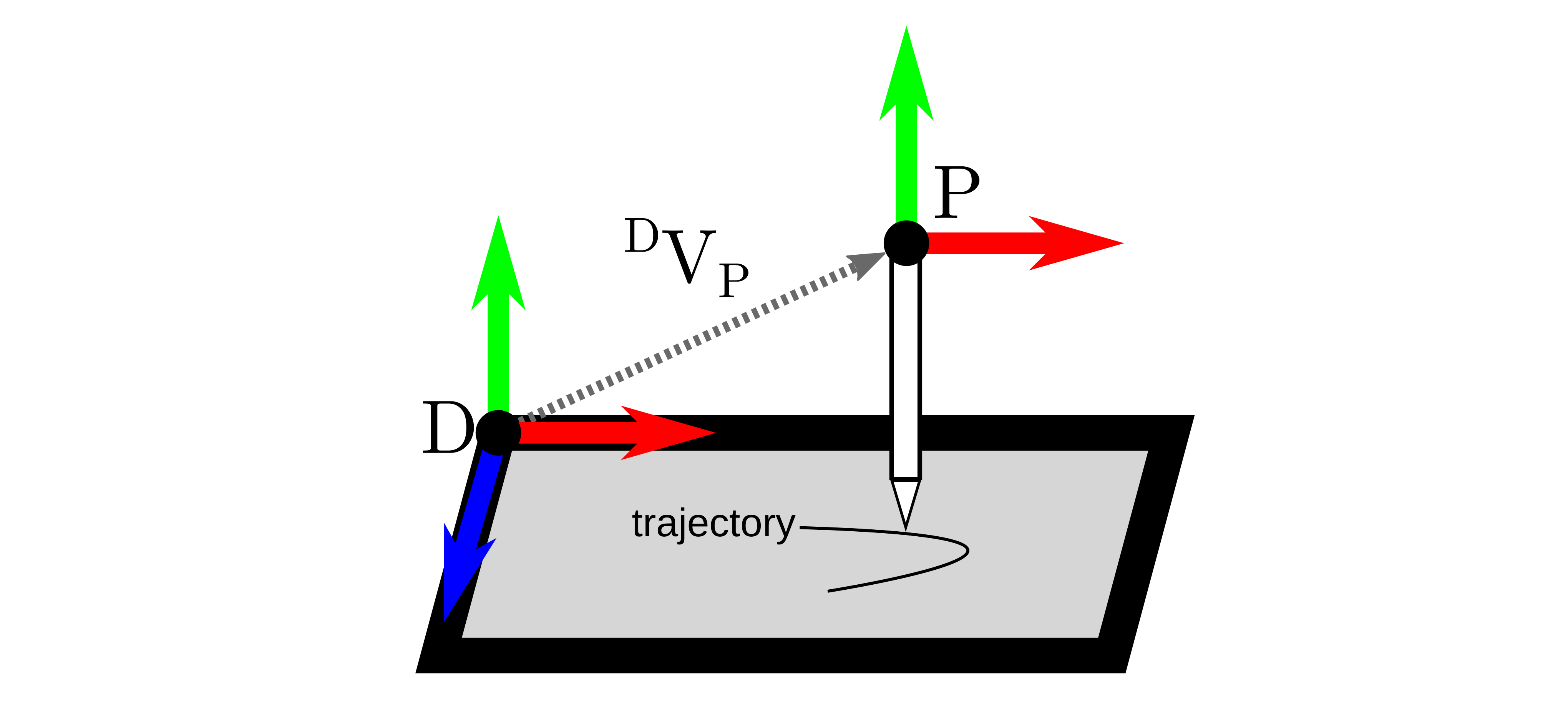
We can assume that the screen corner sits at the origin of the X-Z plane in the $D$ frame, with the touchscreen surface pointing upwards along the +Y direction. Similarly, we can assume the pencil is rigidly attached to the $P$ frame origin, pointing downward along the -Y axis. With $\ell$ as the pencil's length, the tip position is given by the fixed vector $^P\vec{v} = (0, -\ell, 0, 1)$.

$^DV_P$ already describes the relationship between the two frames. Making it time-dependent, $^DV_P(t)$ turns a single target into a full trajectory — a straight line, an arc, a contact-and-sweep profile, whatever the test actually requires:

$$ ^D\vec{r}(t) = {}^DV_P(t) \cdot {}^P\vec{v} $$

Nothing else in the loop equation changes, because nothing else needs to: $^DV_P(t)$ alone is enough to solve for $^RC_E(t)$ — the robot doesn't need to know anything about the probe's internal geometry to be told where to move.

In other words: the robot only ever needs to know where frame P should be. The tip vector is what tells you where the pencil actually goes.

This is where the abstraction pays for itself. Authoring a test now means writing $^DV_P(t)$ in the frame that matches engineering intent — the device — and never in the frame that matches whatever machine happens to be bolted to the bench. Sampling that trajectory at each instant $t_i$ and solving the same loop equation for $^RC_E(t_i)$ produces the exact sequence of robot poses needed to realize it, whether the hardware underneath is a single linear stage or a six-axis arm.

From Robot Control to System Representation

This reframing changes how automation platforms get designed. Hardware is no longer embedded inside the software; instead, the software contains a model of the physical world, and the hardware simply has to conform to it. Robots become interchangeable components. Fixtures become configurations. Tests become hardware-independent descriptions of engineering intent, written once and left alone as the physical rig around them changes.

The result isn't just a more flexible robot controller — it's an automation architecture designed to survive change, in the same way a well-designed API survives a rewrite of what's behind it.

Conclusion

None of the mathematics here is new — chained coordinate transformations are decades-old robotics theory, the same idea behind a ROS tf tree or a set of DH parameters for a robot arm. What's underused is applying it outside robot control, to the validation and test infrastructure built around the robot. The lifespan of that infrastructure shouldn't be dictated by whichever motor happened to be on the bench when it was built. Write software that understands motion, geometry, and intent, and the robot becomes what it should have been from the start: an interchangeable building block, not a dependency baked into every line of test code.

---

¹ Kinematic Modeling and Control of Modular Reconfigurable Robots